Machine Learning
This page serves as a consolidation of notes. The notes are from the "Machine Learning" class given by Standford University on coursera.org. If you want to understand the material yourself, I highly recommend viewing the lectures for that class.
Week 1
Machine learning is the concept of a computer learning something itself without being specifically programmed to do that something.
There are two types of learning. Supervised and Unsupervised.
Supervised learning means we feed the correct answers to the computer. Linear regression (house pricing vs. sq. ft.) and classification (has tumor vs. cell size) are supervised.
Unsupervised learning means we ask the computer to find something for us without giving it a correct answer. Clustering (giving a computer demographics and asking it to separate customers into different markets) is unsupervised.
m is the number of training cases.
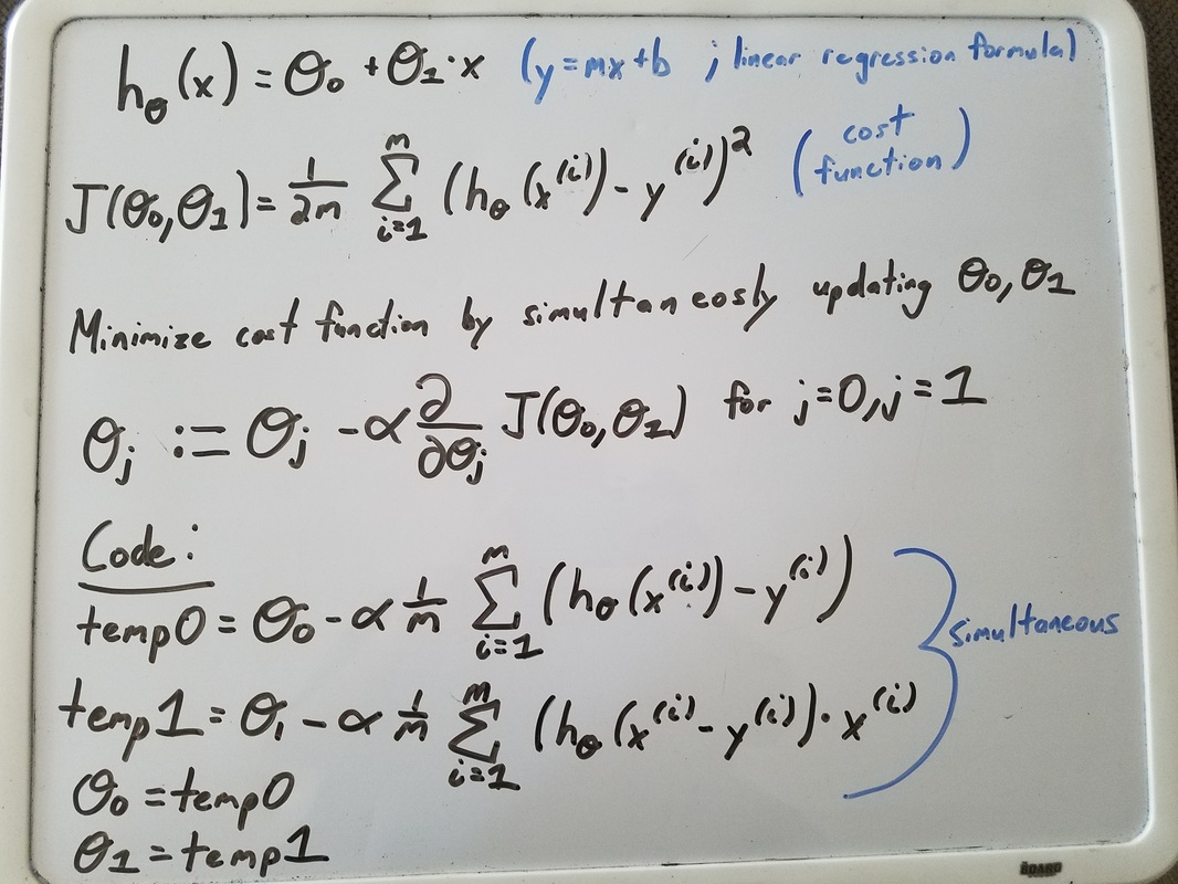
For linear regression, we use the expected y=mx+b formula to try to fit a best line.
We guess the m and b (Theta1 and Theta0) and have a cost function to determine how good our line is, based on how far away our guess for a value is compared to what the actual training data's value is.
Using (Batch) Gradient Descent, we can calculate the correct m and b by guessing initial values, and simultaneously updating m and b by making them slowly move toward a "minimum" in their graph.
Week 2
Multivariable Linear Regression
n is the number of parameters. Like square footage in a house, # of bedrooms, house age, etc. All "features" that go into guessing a price.
x^i means the training case number. (Row)
x_j means the parameter number. (Column)
Usually add a column of 1's at the beginning to pair with Theta 0
h = Theta0*X0 + Theta1*X1 + ... + Thetan*Xn, where X0 is 1.
In matrices, X = [x0; x1; ...; xn] (It's a vector; one column).
Theta = [Theta0; Theta1; ...;Thetan] same as X.
h = Theta' * X; (Theta' = Theta transpose)
For alpha choosing, start with something like 0.001 -> 0.003 -> 0.01, etc. Go up 3 fold each time. If alpha is too big, the gradient descent won't converge. If it's too small, it'll take a long time.
For normalization, we want features to be around the same scale. Get the mean of everything in the column (feature), get the standard deviation. For each training case in that column, subtract the average and divide by the standard deviation. For each future guess we want to use the regression to check, we have to normalize it, so keep the average and standard deviation stored.
To debug, plot J vs. the number of iterations to check if J decreases each time. Or else adjust alpha.
The normal equation can be used like gradient descent, and is good if n is less than 10,000. Otherwise it takes a while to calculate. It's completely analytical. Meaning it's a straight calculations.
Theta = pinv( X' * X ) * X' * y
Gradient descent is the same as before, but keep the x_j to multiply with.
How to do it:
1. Pick the number of iterations gradient descent runs for, and your alpha value.
2. Have a file for calculating the cost function.
3. Have a file for calculating the gradient descent.
4. Have a file for normalizing variables.
5. Have a file for stringing everything together, including loading the data.
As an example, see the following file that was homework for Week 2:
| machine-learning-ex1_done.zip | |
| File Size: | 506 kb |
| File Type: | zip |


